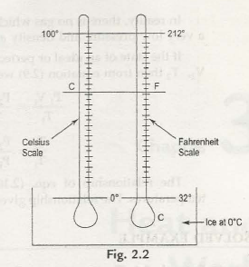
The introduction to temperature measurement is well explained by the zeroth law of thermodynamics. Therefore to gain a measure of temperature a reference body whose characteristics are known to us with all probable changes in temperature. This is called the thermometric property, and the reference body is referred to as a thermometer. We are aware that in conventional thermometers Expansion of mercury is utilised. A table is given below table 2.1 which lists the type of thermometers along with its property.
Table 2.1
- No Thermometer Thermometric property Symbol
- Mercury-in-glass Length L
- Constant volume gas Pressure p
3 . Electrical resistance Resistance R
- Constant pressure gas Volume V
- Thermocouple Thermal Electromotiveforce E
- Pyrometer (Radiation) Intensity of radiation I or J.
2.2.1 Empirical Relations between Temperature and Thermometric Property
Let us consider that x be the thermometric property and temperature of a linear function (straight proportionality) of x. So, arithmetically we get,
f(x) = nx
where a is a random constant.
If x1resembles to f (x1), then x2 can be calculated as follows.
f(x1) = ax1
a = f (x) / x1 inserting this in equation (2 .1 ) we get
f (x) = f (x) / x1 .x
x = x2 we get from (2.2)
f (x2) = f (x1) / x1 . x2
f (x2) / f (x1) = x2 / x1
Equation (2.3) displays that two temperatures on the linear x scale are as the proportion of the analogousanalyses i.e., x2 and x1.
2.2.2 Method Used Before 1954
Let us assume, f(x) = ax + b … (2.4)
At first the thermometer is located in connection with a standard system and the temperature is thus measured. Let us consider x1 as the reading, therefore:
f (x1) = ax1 + b
nowthe thermometer is measured with other standard systems and let us consider the temperature as x2, so we get:
f (x2) = ax2 +b
Solving (2.5) and (2.6) for a and b,
F(x1) – (x2) = a (x1 –x2)
A = f (x1) – f (x2) / x1 –x2
(2.5) => b = f (x1) – ax1
= f(x1) – f(x1) – f(x2) / x1 – x2 .x1
= x1 f (x1) – x2 f (x1) – x1 f( x1) + x1 f (x2) / x1 –x2
b = x1 f (x2) – x2 f(x1) / x1 –x2
now putting the value of a and b in (2.4), we get
F(x) = f(x1) – f(x2) / x1 –x2 .x + x1 f(x2) – x2 f (x1) / x1 –x2
Note : If b = 0 then equation (2.7) decreases to
F(x) = f(x1) – f(x2) / x1 –x2 .x
and we obtain b = 0 = x1 f(x2) –x2 f (x1) / x1 –x2)
The two most commonly used scales of measure are Celsius scale (C) and farenheit scale (F). there was two fixed points which was used as steam points( boiling point) and ice points (freezing point) before 1954.
Temperature Celsius scale Fahrenheit scale
Steam point 100 212
Ice point 0 32
Interval 100 degrees 180 degrees
100 -0 /C -0 = 212 – 32 /F -32
100 / C = 180 / F -32
5 /C = 9 / F -32
C /5 = F -32 / 9
2.2.3 Method in Use On and After 1954
However, after 1954, Kelvin recommended that there be one fixed point which is important to create a temperature scale. The triple point of water can also be considered as a fixed point. The value of a triple point is 0.01oC or 273.16 K. Individually, the ice point of 0 o c on Celsius scale and if converted then it becomes 273.15 K on Kelvin scale.
Let us consider to C as Celsius scale and T for Kelvin scale.
Then we get,
Tin Kelvin= 273.15 + to C.
The triple point of water on the Fahrenheit scale is 32.02F
for Rankine scale is 491.69R
T in Rankine scale = 459.67 toF
Table 2.2
Fixed point Celsius Kelvin Falzrenlieit Rankine
Steam point 100 373.15 212 671.67
Triple point of water 0.01 273.16 32.02 491.69
Ice point 0 273.15 32 491.67
Absolute zero – 273.15 0 – 459.67 0
Links of Previous Main Topic:-
- Force mass acceleration
- Simple stress introduction
- Normal strain
- Statically indeterminate system
- Introduction to thermodynamics
- Statement of zeroth law of thermodynamics with explanation
Links of Next Mechanical Engineering Topics:-
- Heat and work introduction
- First law of thermodynamics for a control mass closed system undergoing a cycle
- Open system and control volume
- Conversion of work into heat
- Introduction to carnot cycle

