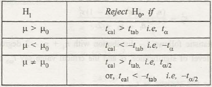
(a)Test of a Single Mean. Here sample is small which (n < 30) and cr is unknown
- Setting up H0 : µ = µ0 2.
- Set up H1 : µ > µ0 or µ < µ or µ ≠ µ0
- Test statistic
t = ~ t
Distribution with (n – 1) degrees of freedom
- Setting up level of significance denoted by the a and the critical value is denoted by the !tab (from table of t – distribution).
- Computation of the statistic saytcal
- Decisions
| H1 | Reject H0, if |
| µ< µ0 | tcal>ttabi.e., tα |
| µ > µ0 | tcal<-ttab i.e., -tα |
| µ ≠ µ0 | tcal<ttab i.e., tα/ 2
Or, tcal>-ttab i.e., -tα/ 2 |
All ttab based on (n – I) which is the degrees of freedom.
Example 5:
The mean breaking strength of a certain kind of metallic rope is 160pounds. If six pieces of ropes (randomly selected from different rolls) have mean breaking strength of 154.3 pounds with a standard deviation of 6.4 pounds, test null hypothesis 1…1. = 160 pounds against the alternative hypothesis 1…1.<160 pounds at 1% level of significance. Assume that the population follows normal distribution.
Solution:
- H0: µ= 160 pounds
- H1: µ< 160 pounds
- Since n = 6, Here the test statistic is considered as
t=
- α = O.OI,
H1 indicates that it is left tailed test. Critical value is 6- 1 which is 5 degrees of the freedom is -3.365
- Computation
tcal == –2.18
- Decision
Since tcal> -3.365
- It is located in the acceptance region
- H0 is accepted
- The Mean breaking strength of the metallic rope is considered as I60 pounds.
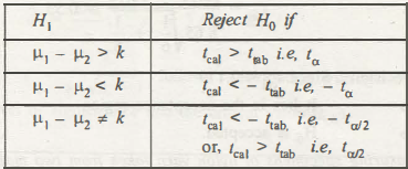
- b) Testing of Difference of Two Means. In this n1 and n2 are small (< 30) and the population variances are not known but equal and two populations are followed by normal distribution.
- Setting up H0 : µ1- µ2 = k
- Setting up H1 : µ1- µ2 > k, or µ1- µ2 < k or µ1- µ2 ≠ k
- Test statistic
t =
Here, the statistic is followed by t – distribution with n1 + n2- 2 degrees of freedom.
- Setting up of level of significance, a. and the critical value say t13b at n1 + n2 – 2 degrees of freedom.
- Computation of test statistic as tcal·
- Decision
| H1 | Reject H0, if |
| µ1 – µ2 < k | tcal>ttab i.e., tα |
| µ1 – µ2> k | tcal< -ttab i.e., -tα |
| µ1 – µ2 ≠ k | tcal<-ttab i.e., -tα/ 2
Or, tcal>ttab i.e., tα/ 2 |
Example 6. The following are the number of sales with a sample of 6 sales people of gas lighter in a city A and a sample of 8 sales people of gas lighter in another city B made over a certain fixed period of time :
City A : 63, 48, 54, 44, 59, 52
City B : 41, 52, 3850, 66, 54, 44, 61
Assuming that the populations sample is closely related with normal distributions which is having the same variance, test H0 : µ1 = µ2 against H1 : µ1 ≠ µ2 at the 5% level of significance.
Solution
- H0 : µ1 = µ2
- H1 :µ1 ≠ µ2
- Test statistic:
Links of Previous Main Topic:-
- Introduction to statistics
- Knowledge of central tendency or location
- Definition of dispersion
- Moments
- Bivariate distribution
- Theorem of total probability addition theorem
- Random variable
- Binomial distribution
- What is sampling
- Estimation
Links of Next Statistics Topics:-
- Statistical hypothesis and related terms
- Analysis of variance introduction
- Definition of stochastic process
- Introduction operations research
- Introduction and mathematical formulation in transportation problems
- Introduction and mathematical formulation
- Queuing theory introduction
- Inventory control introduction
- Simulation introduction
- Time calculations in network
- Introduction of game theory


