Bivariate Distribution can be described best by mentioning the region of two Cartesian planes such as, x-y. In this two-dimensional array, when two variables are found to be continuously random then they are bivariate. If variables can reach above the interest level upon that two-dimensional plane then that is specifically known as probability density. The function of this density is related with bivariate distribution.
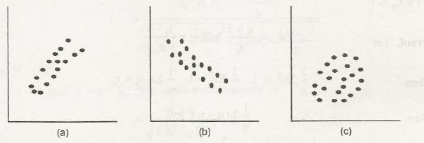
The bivariate distribution is explained through a diagram called scatter diagram. The above statement can be explained as:
For example, we are taking X and Y to be the random valuables where we are taking x and y as their values, the two-dimensional Cartesian plane as R. So when we try to reach to the probability density then we come to: fxy(x,y). So when we try to reach the surface of R of this density and its function we come to:∫∫R fxy(x,y)dr dy =1
The variables of bivariate distribution may have positive or negative correlation. In the positive correlation, the decrease or increase of one variable will cause the decrease or increase of that other variable. In the negative correlation, the decrease or increase of one variable will cause the increase or decrease of that other variable.
Links of Previous Main Topic:-
- Introduction to statistics
- Knowledge of central tendency or location
- Definition of dispersion
- Moments
Links of Next Statistics Topics:-
- Theorem of total probability addition theorem
- Random variable
- Binomial distribution
- What is sampling
- Estimation
- Statistical hypothesis and related terms
- Analysis of variance introduction
- Definition of stochastic process
- Introduction operations research
- Introduction and mathematical formulation in transportation problems
- Introduction and mathematical formulation
- Queuing theory introduction
- Inventory control introduction
- Simulation introduction
- Time calculations in network
- Introduction of game theory

