Chapter 4 – Individual and Market Demand

4.1 Individual Demand

With a fixed budget allocation, consumers choose goods and amount of goods to maximize utility. Consumers’ demand for goods varies according to prices, prices of other goods and income. A useful tool for analyzing demand behavior – individual person’s demand curve depends on choice of goods for consumption which that person makes.

The analysis will be done graphically considering food and clothes as goods.

Price Changes

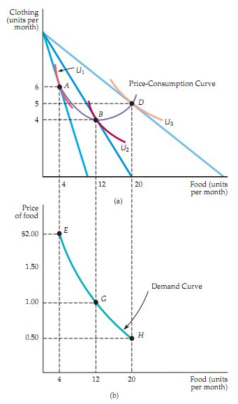
It is interesting to note how consumption of two goods change when price of one good changes. Figure 1(a) depicts a typical Price-Consumption Curve. Point B represents the utility-maximization consumption choice of the consumer, when price of food is $1. U₂ is the corresponding indifference curve.

Figure 1(b) represents individual demand curve. It shows the demand of quantity of goods corresponding to price of good. Point G corresponds to point B in figure 1(a).

If price of food is raised to $2, the consumer utility-maximization consumption choice moves to point A. On the demand curve, the consumer’s position changes to point E as demand of food units reduces with the rise in price.

The budget line which is tangent to the indifference curve also rotates inwards about the vertical intercept. Now if price of food is decreased, consumer can purchase more units of food. Utility-maximization choice moves to point D. On the demand curve, the consumer’s position

Figure 1

position changes to point H.

The Individual Demand Curve

It is evident that this price-consumption curve plots different utility-maximizing blending of clothes and food at different prices of food. As price of food reduces, consumer can buy more units of food. Consumption of the other good, i.e., clothes can increase or decrease as this process is carried on. In other words, the purchasing power of consumer changes with the change in price of any good.

With individual demand curve, you can relate the quantity of any specific good that any single consumer will buy that good.

Important properties of individual demand curve:

1. Individual demand curve shows the changes in utility level in relation to change in price of good.
2. The aim of consumer is to maximize utility within the budget constraint. In technical terms, consumer’s choices must satisfy that condition where MRS or marginal rate of substitution of food for clothes is equal to the ratio of the prices of food and clothes.

(MRS) is the measure of maximum amount of one good that an individual agrees for giving up his one good to obtain a single unit of other good.

On demand curve MRS of food and clothing decreases with the decrease in the value price of food.

Income Changes

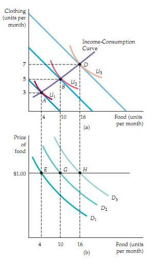
Consumption pattern of people also changes with change in income. In figure 2(a) we’ve shown income-consumption curve at three different income levels. Initially when income of person is $10, optimal choice of consumer is A. Keeping the price of food fixed at $1 we see point E as consumer’s choice on demand curve in figure 2(b).

As the income is increased, in figure 2(b), budget line of consumer moves outward parallel to original budget line. Correspondingly, the utility-maximization choice of consumer also changes.

While analyzing price change we saw a shift in consumer’s choice on the same demand curve. Here as income changes, demand curve itself shifts to the right.

Figure 2

Normal Goods versus Inferior Goods

As seen in figure 2, slope of income-consumption curve is positive. This implies that quantity demand increases with increase in income. Income elasticity of demand is also positive.

Income elasticity of demand is the percentage change in quantity demanded resulting from 1% change in income. If demand curves shifts to the right more with income rise then income elasticity is also more. Goods with such behavior are called normal goods. In other words, people have a tendency to buy greater amount of normal goods when income rises.

However, there are certain goods whose demand falls with income rise. These goods are termed inferior goods and these have negative elasticity of demand.

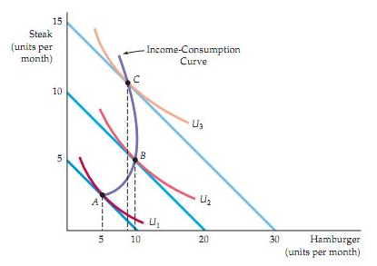
Figure 3 shows income-consumption curve for inferior goods. For certain income levels, both steak and hamburger are normal goods but when income rises above a level, hamburger becomes an inferior product. Here, income-consumption curve bends inwards.

Figure 3

Engel Curves

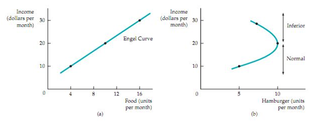
If we plot quantity of goods in relation to income level of consumers, we obtain Engel curves. For normal goods, demand of goods increase steadily with the rise in income. Hence the upward slopes of the Engel curve as in figure 4(a). All normal goods like food and clothing will have positive sloped Engel curves.

Engel curves for inferior goods have opposite slope. This indicates that demand for inferior goods lowers after certain level of income rise.

Figure 4

Example of Consumer Expenditures in US:

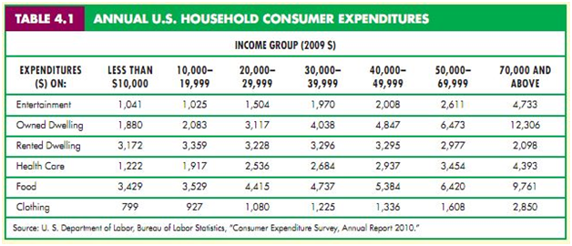
Engel curves can be applied to study consumer expenditures across various income groups. Table 1 lists average spending on various goods of US consumers of different income levels. The data has been compiled by US Bureau of Labor Statistics.

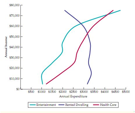
Goods like food, clothing and healthcare show normal behavior, as consumption increases with the rise in income level. However, people with low income prefer to spend more on rented housing rather than owning houses, while high income consumers spend more on owned houses. This pattern shows that rented housing is inferior good.

Figure 5 shows Engel curves for Entertainment, Rented Dwelling and Health Care. Curves for Entertainment and Healthcare have a positive slope almost throughout the span of income levels. But for Rented Dwelling, the Engel Curve bends inwards for higher income groups.

Figure 5

Substitutes and Complements

While plotting demand curves, price of one good is kept fixed and behavior of utility-maximization is analyzed on the basis of change in price of other good. However, in real world, demand of goods might depend on price of other products.

Some goods are used together. For instance, computer hardware and software, baseball bats and balls, and shoes and socks. There are also goods which act as substitutes for other goods. Diet cola substitute for cola, movie tickets for DVD rentals and so forth.

Here, an example can be taken. Let us say that cost of a specific movie ticket rises, so it is expected that more videos would be rented since videos and movie tickets are taken as substitutes. Similarly, when two products are complement to each other, increase in the price of one product leads to a reduction in quantity of the other. Say, gasoline price is raised resulting in low consumption of gasoline, motor oil consumption would also fall since both these are used together. Hence, two products are said to be independent if price of one product has no effect on quantity demanded of the other product.

Goods can be substitutes or compliments on different occasions. Real time market situation dictates the way demand of one good behaves due to change of price of other goods. It becomes a little complex in determining if goods are substitutes or compliments given the fact the a large number of goods are prevalent in the market.

4.2 Income and Substitution Effects

Figure 6

Fall in prices have two main effects:

1. Substitution effect: Consumers have a tendency to buy more quantity of cheaper goods and less of more expensive goods.
2. Income effect: Actual purchasing power of consumers increase with fall of price in certain goods. As a result, demand for other goods also rise.

Substitution Effect

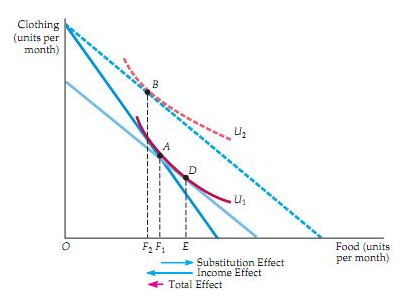
When price is dropped, both substitution and income effect comes into action. Substitution effect is known as change in consumption of food products with change in price of food where utility level is taken as consistent. Since, this change in consumption is associated with change in price hence food becomes comparatively cheaper than clothes.

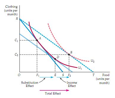
This movement in substitution is marked via an indifference curve. In this case, in Fig 6, this substitution curve can be found by drawing a budget line that is parallel to new budget line that has already been drawn, RT, depicting lower relative price of the food products). This curve is tangent to original indifference curve that is taken at U1 (this act as standard of satisfaction level).

This new imaginary budget line that is placed at lower level is used for understanding that there was a reduction in nominal income for getting to the conceptual goal of substitution and isolating effect. If that budget line is taken consumer wants to have D as the market basket and has OE unit of food products. So, F1 E line segment is taken for representing substitution effect.

Income Effect

If the income effect is taken into consideration, it can be seen that, with increase in purchasing power there is a change that is brought about in consumption process. In Fig 6, it can be seen that income effect is depicted by moving from imaginary budget line which passes through D and cuts parallel budget line RT, which has passed via B. If consumer chooses basket B on U2 indifference curve, there is increase in consumption level from OE to OF2. This is taken as positive income effect and since it is a normal good so these movements from a single indifference curve to another, results in measuring change that a consumer has made in terms of purchasing power. It is seen in Figure 6 that theoretically, total effect of price change is summation of both income and substitution effects.

Total Effect (F1F2) = Income Effect (EF2) + Substitution Effect (F1E)

The substitution effect always has the same direction, where decrease in price rates results in an increase in consumption rates. But there are chances that income effect can change demand of a consumer in case that concerned good is inferior or normal. So, with an inferior good income effect turns into a negative value. As income rises, consumption falls. Figure 7 indicates the income and substitution effects for inferior good. The line segment EF is used for showing this negative income situation. Also, with inferior goods substitution effect is larger than income effect. So, with their price decrease, consumption increases.

Figure 7

Figure 8

A Special Case: The Giffen Good

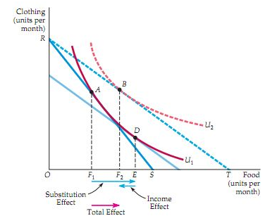
Speaking on a general note, income effect has the power to ensure that demand curve of specific good slopes in an upward direction. This kind of good is called a Giffen good with Fig 8 showing both income and substitution effects. It is taken that a consumer is at A, with less clothes and food being consumed by him. Now with a fall in price of food products, enough amount of income is left that can be used for buying of clothes and less amount of food. This is depicted by B. so, technically, consumer is better at B rather than A though amount of food is less in comparison to A. Giffen goods as a matter of fact has negative income effect. So, these goods take up a small part of consumer’s income. When it comes to larger incomes, normal goods are taken into consideration.

4.3 Market Demand

Having studied the demand behaviors of individual consumers, we can sum up all individual patterns to derive market demand in a particular market.

From Individual to Market Demand

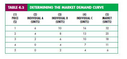
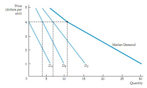
In figure 10, we see demand curves of three customers A, B and C for coffee, represented by D_A, D_B and D_C. For every price of coffee, market demand curve is obtained by adding up individual quantities purchased by A, B and C. For example, when price of coffee is $4, A buys no unit, B buys 4 units and C buys 7 units. Sum total of the three is 11, which gives the point on the market demand curve. The other points on market demand curve can be obtained in the similar process.

Market demand curve is kinked at one point as A does not make any purchase at one price of coffee.

Market demand curve shifts more towards the right as more customers are added to the market.

As the market demand curve is a simple summation of individual demand curves, any change in the behavior of individual demand curves also affects market demand curve. As we have seen in previous sections, change in income shifts the demand curve of consumers. This change will also result in shifting of market demand curve as well.

Figure 10

Elasticity of Demand

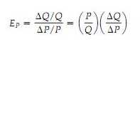
Price elasticity of any demand measures the percentage change in quantity demanded that will be resulting from the 1% increase in price. If quantity of a good is stated by Q and its price by P, then price elasticity of demand becomes

Inelastic demand: When E_P is less than 1, the demand is said to be inelastic. The quantity demanded does not change due to a change in price.

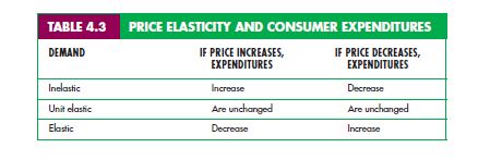
Elastic demand: When E_P is greater than one, demand is elastic. And, the total expenditure on good decreases as this price goes up.

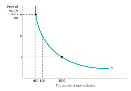
Is o elastic demand: If price elasticity of demand is constant all along demand curve, we can say the curve is is o elastic. The figure 11 depicts is o elastic curve.

Figure 11

Speculative Demand

In real world, demand of some goods depend not on actual consumption but on the speculation that the prices will rise in future and hence consumers purchase the goods without any consumption needs. This behavior of consumers is irrational. People tend to purchase goods in speculation with the idea of reselling the goods when price rises.

Real estate and housing sector sees the most speculative demand. Consumers have a common idea that house prices keep on rising and as a gamble, they buy or book housing to resell it later.

Links of Previous Main Topic:-

• Introduction Markets and Prices Preliminaries
• The Basics of Supply And Demand
• Consumer Behavior
• Appendix to Chapter 4 Demand Theory a Mathematical Treatment

Links of Next Microeconomics Topics:-

• Consumer Surplus
• Uncertainty and Consumer Behavior
• Production
• The Cost of Production
• Production and Cost Theory   A Mathematical Treatment
• Cost in the Long Run
• The Cost of Production Production with Two Outputs
• Profit Maximization and Competitive Supply
• The Analysis of Competitive Markets
• Market Power Monopoly and Monopsony
• Monopolistic Competition and Oligopoly
• Game Theory and Competitive Strategy