4.4 Consumer Surplus

Consumers buy products to satisfy their needs and to get some utility. They pay some price for it. Now, when one buys a commodity, he loses some utility while paying for it. Different consumers decide price of a particular product according to their will. Thus a contradiction occurs about the maximum price (i.e. willing by customers) of a product. Consumer surplus calculates this gap. The aggregate consumer surplus includes all customers’ data in the market.

A simple instance can make this concept clear. Suppose that a girl wants to buy a ticket to rock concert showand has been willing to pay $ 13 for it. But she actually paid $ 12 after buying it. Here, ($ 14 – $ 13) = $ 1 is the surplus.

Consumer Surplus and Demand

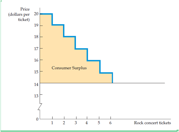
Consumer surplus has an easy definition. It is the difference between what a consumer is willing to pay and what is actually paid. The demand curve is the graphical way to measure consumer surplus. Consider the example of the ticket price. Astair case-like structure is made here for easy understanding.

In the following graph, calculations are made on consumer surplus, associated with six tickets; price of each is $ 14 marked by a yellow shaded area.

Figure 4.14

While deciding how many tickets to buy, the girl may think about the following facts. The first ticket’s price is $ 20, but she has to pay only $ 14. So, $ 6 is the surplus. For the second ticket, she pays only $ 15 instead of $ 20. Likewise, for the third, the surplus is $ 4. In this way, when she buys the sixth ticket, it goes down to $ 1. Buying a seventh ticket is no profit, no loss. Thus the total surplus is:

$6+$5+$4+$3+$2+$1= $ 21

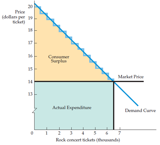
Now, it is an individual’s demand curve. When thousands of consumers in a market are considered, it is impossible to count the demands of all. So, the demand curve is like a straight line. Here, the actual expense is 6500* $ 14 = $91,000. Calculation for the yellow shaded area is,

½ * ($ 20 – $ 14) * 6500 = $ 19,500

 Fig 4.15

4.5 Network Externalities

In a market, there lies a mutual network between a consumer and a commodity. Demand for a good and utility are the key factors of this network. But this process is not one is to one. An individual’s demand leaves an impact on others purchasing. It is applicable for some goods. And here starts the network externality. It is like a cause and effect system.

While working with market demand curve, we always assume that an individual’s demand is unaffected by others; like, a person’s consumption of coffee perfectly depends on his own choice, taste, price etc. Thus, we draw a horizontal demand curve.

However, in reality, the situation is different. Network externality is present and one’s demand touches on others. There are two types of externalities, they are Positive and Negative.

Positive Network Externalities

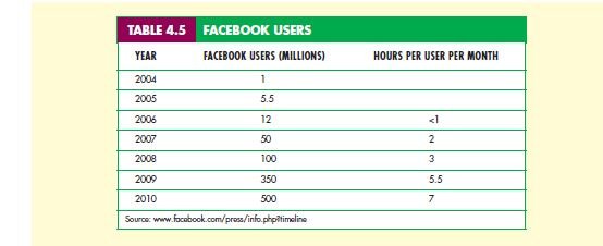
A couple of examples from real life can clarify the concept of Positive Network Externality. An increasing craze for social networking site can be a good example of Positive Network Externality. People gets attracted as their peers use these social networking sites and the number of users thus increase day by day. The internet connection is a must for this. Here, to get connected with others, people starts to use the internet; thus leaving an impact on one another’s demand.

• Bandwagon Effect – It can be called a product of Positive Network Externality. It occurs when a consumer imitates other consumers in a society. As a result, the market demand curve becomes flattered or becomes more elastic. A child wants to have the same toy that all other children have around him/her. People buy apparels which they see others are using to follow the current style trend. Bandwagon Effect has a great impact on price determination in a market.

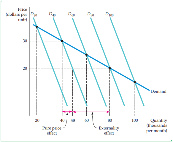
Figure 4.17 depicts the Positive Network Externality. Here, the count starts with 20,000 people who have bought a certain product. Compared with the total population, it is a very small value. The demand is indicated by D₂₀ here. Then, suppose the demand increases; now those people who are going to buy that product also gradually increase (40,000 to 60,000 to 80,000 and so on). The demand curve shifts towards right and demand are indicated by D₄₀, D₆₀, and D80 etc. In this figure, it is observed that as an effect of the price drop ($ 30 to $ 20), it became more elastic.

Fig 4.17

Negative Network Externalities

Congestion offers are perfect examples of Negative Network Externalities. In an amusement park or a skating rink, the price gets lower when more people buy tickets.

• Snob Effect–The Snob Effect arises when a section of people of a society desires to own unique and costly goods, like rare artworks, exclusively designed cars etc for exhibiting status and prestige.

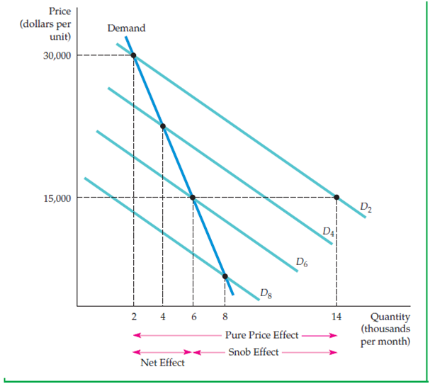
Figure 4.18 explains the Snob Effect. The demand curve here becomes steeper or less elastic.

Fig 4.18

Consider the demand curve D₂. When there are only 2000 buyers, the price is comparatively high. But when the curve shifts towards D₄, D₆ and finally D₈, that means the number of buyers is increasing and the price is decreasing. In Snob Effect, if the price is $ 30,000; there will be 2000 buyers. But when the price lowers to $ 15,000, customer response will be less. The value of the product will be less for them. Here lies the effect of Negative Network Externalities. Think about Rolex watches; a high price is charged for creating snob effect.

4.6 Empirical Estimation of Demand

In this section, a discussion is presented about how consumer’s demand bears upon an economic firm’s decision of marketing. Their approach towards their customers is determined by studying the demand curve, its shifts, and elasticity. For instance, General Motors decides their customer policy (providing loans or rebates) depending on consumer’s demand. In a country, the government ascertains public policies after checking demand. This discussion will help students to gain knowledge about consumer behavior.

The Statistical Approach to Demand Estimation

An actual study of demand, i.e. the direct market study is immensely important for a business organization. They sort out their demand estimation through statistics and build their market strategy.

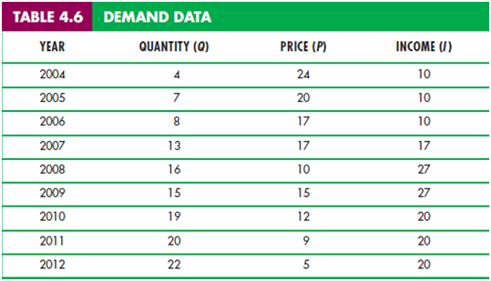
In Table 4.6, this statistical approach is shown through an example. It represents the demand data of Raspberries in the market. The quantity, price, and income of different years of this organization are given. It is presupposed that to predict the demand determination, the researchers detected that raspberry production is weather sensitive; the current market price has no effect.

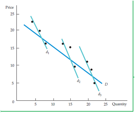
Figure 4.19 is a graphical representation of this table. It describes the demand relationship.

Fig 4.19

We can draw a simple straight demand curve if we there are no other determinants of demand. Q = a – bP, that will be the equation for the point. If the demand is unaffected by other factors than price, then only the curve D (equation: Q=28.2 – 1.00P) is appropriate.

Here in this study, the income (I) is increased twice, so the demand curve is shifted two times also. These shifts are parallel. The linear demand curve equation is

Q = a – bP + cI

The demand relationship is calculated by the least square method. It is,

Q = 8.08 – .49P + .81I

The Form of Demand Relationship

The demand curve is a straight line when the price does not affect the quantity demanded. But when it varies with the price level, the equation is like this:

For the demand equation Q = a – bP, the price elasticity Epwill be

Ep= (Q / P) (P/Q) = -b (P/Q)

As a result, the elasticity and price increase and the quantity demanded decreases.

If we consider the Table 4.6, the approximate linear demand for raspberries can be calculated like this:

Q = 8.08 – .49P + .81I

Now, it can be observed that the elasticity of demand in 1999 is:  – .49(10/16) = – .31 [Here Q= 16, P = 10]. On the other hand, in 2003 this elasticity has been decreased to -.11 [Q=22, P=5]

For adapting easy method of calculation, in the is o elastic demand curve, the price elasticity and income elasticity are supposed to be constant. Here is the log-linear form of is o elastic demand curve:

log (Q) = a – b log (P) + c log (I)

It is a logarithmic function, where a, b, c are constants where ‘b’ denotes price elasticity of demand and ‘c’ is income elasticity.

From Table 4.6, we obtain the following equation of linear regression:

log (Q) = – 0.23 – 0.34 log (P) + 1.33 log (I)

The values 0.34 and 1.33 are the price elasticity of demand and income elasticity for raspberries respectively.

While studying about complementary goods and substitute goods, the following demand function can be presented:

log (Q) =  a – b log (P) + b2 log (P2) + c log (I)

Here, P₂ is a product which is related to the main product we are working with and b₂ is the cross price elasticity. If b₂ is positive, two goods are substitutes; otherwise, its negative value denotes two goods are complementary.

Working with demand curves is a must for all economic and marketing experts for regulating a business. They use supermarket scanner data as inputs for studying the demand relationship. After determining the price elasticity of demand for a particular product, it becomes easy for a firm to fix the price of that product. The profit for a product increases with the degradation of magnitude of elasticity.

Interview and Experimental Approaches to Demand Determination

As the civilization is growing, the need of human is increasing; and it is almost impossible for a company to know individual’s demand. A company thus sets its market strategy by assuming different ways. Interview of customers is a process to find out the approach of a customer towards a product and what price they are willing to pay for it. But economists have pointed out some drawbacks of this method. People cannot always know every details of a product; therefore they may take less interest in this kind of interview. To eradicate this problem, interviewers often take a roundabout way in a survey. Discounts and offers are given on a product to observe the customer behavior.

It is a bit long term process actually. For example, one can think of the airline’s company. They sometimes offer tickets at a reduced price. Hence, they have two main objectives: to examine if there is any change in ticket purchasing and the strategies of other competitors in market.

Now, this experiment should be continued for certain months to identify the change in the demand curve. Then only an enterprise can count its benefit. However, many other factors are entangled with this kind of experiment. People’s choice for a product may completely change. So, even if this interview method is conjectural, to count profit and loss of a company and demand determination, this method can be applied only a few times.

Summary

1. Taste of goods and budget limit of the individual customer are some factors to construct individual’s demand curve.
2. To distinguish the relation between how much good is consumed and income of a consumer; Engel’s curve is used. It explains how consumer’s expenditure varies with income.
3. For complementary goods, when the cost of one increases, then the demand of other will decrease and vice versa. For substitute goods, the price and demand increase simultaneously.
4. Changing price for quantity demanded is of two types. A) Substitution effect – the utility remains unchanged with price change B) Income effect – the price is constant with utility change. For Giffen goods, the price elasticity is positive and income elasticity is negative. It is a special kind of inferior good for which demand curve is upward sloping.
5. The horizontal market demand curve can be used to evaluate people’s consumption of goods and service.

 

Price	Quantity Demanded	Elasticity of Demand	Effect
1 percent increase	Less than 1 percent decrease	Demand is price inelastic	Consumer expenditure increases
1 percent decrease	More than 1 percent decrease	Demand is price elastic	Consumer expenditure decreases
1 percent increase	1 percent decrease	Demand is unit elastic

 

7. Consumer surplus is the difference between the price that people wills to pay and that they actually pay. It is a determinant of customer benefit.
8. For speculative or notional demand, not the direct benefit, but the anticipation of price increase satisfies a consumer.
9. When one consumer’s demand directly affects other’s demand and buying decisions, a network externality arises. It can be either positive or negative. When a customer starts to use a product after seeing many people has opted for it, positive network externality occurs. On the other hand, when a consumer uses a product after noticing that a few people around are using the same, it is negative network externality.
10. Direct marketing approaches like taking interview of the consumers can be beneficial for an enterprise to examine the demand of a product. But, before accepting this process, the researchers should be aware of the authentication of data.

Questions for Review

1. State the difference between the given terms:
   A. Demand curve and Price consumption curve
   B. Individual demand curve and Market demand curve
   C. Demand curve and Engel’s curve
   D. Income effect and Substitution effect

2. A person spends his/her entire money for buying two types of goods, food, and clothing. Find out if both goods are inferior or not with an explanation.
3. Study the following statements and examine if they are true or false.
   A. When one moves downward along the demand curve, the marginal rate of substitution decreases.
   B. The level of utility increases when one moves downward towards the demand curve.
   C. Engel curve is always upwardly sloped.

4. Suppose that a rock concert ticket costs $ 10. The demand for tickets is greater than the availability. What will be the value or marginal benefit for an extra ticket? (>$10, <$10, =$10) State the process.

5. Determine the complementary goods and substitute goods from the given pairs. Can they be either if the circumstances change? Discuss elaborately.
   A. A mathematics class and an economics class
   B. Tennis balls and tennis racket
   C. Lobster and steak
   D. Having a plane trip and a train trip to the same place
   E. Bacon and eggs

6. Notice the example carefully and give explanations.

A person spends a fixed part of his income per month for the following consumptions.

A. Tortilla chips and salsa
B. Tortilla chips and potato chips
C. Buying movie tickets and gourmet coffee
D. A bus trip and travel by subway

              Now, explain how the demand changes with the increase of price. Also, identify which among these pairs are complements and which are substitutes.

7. Point out which of the following situations will cause i) movement along the demand curve ii) shift of the demand curve.
   A. Dismissal of quotas on the import of foreign apparels
   B. The increment of income of U.S citizens
   C. Decrease of industry’s costs for the production of domestic clothes, that is considered as lowering price in the market

8. A. Salt
   B. housing
   C. theater tickets
   D. food

Which of the above goods will show substitution effect with the increase of price?

9. Suppose that an average consumption of gasoline for a household in a state is 800 gallons per year. In a new policy, 20 percent gasoline tax has been brought out along with $ 160 yearly discount for each household. What will be the effect? Does the new program bring betterment or will it worsen the situation?

10. If we consider the price-elastic demand for membership in the Association of Business Economists, which among these three groups will have the most and the least?
    A. Students
    B. Junior executives
    C. Senior executives

11. Examine which of the following pair is more price elastic.
    A. A consumer’s demand for a specific brand of toothpaste and demand for toothpaste in general
    B. The demand for gasoline for a limited period and demand for a relatively long period

12. Define the differences between positive and negative network externalities. Provide examples for each.

Exercises

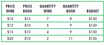
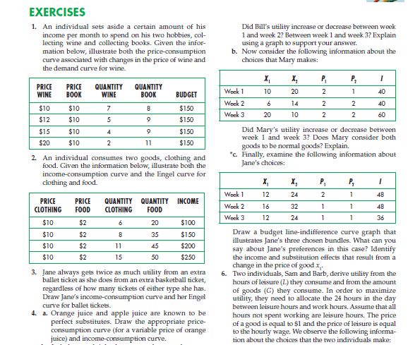
1. 1. An individual spends a certain part of his income for collecting books and collecting wine. Study the information below and draw both the price-consumption curve for the price change of wine and the demand curve for wine.

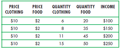
2. 2. Illustrate both the Engel curve and income-consumption curve based on a person’s consumption of clothing and food. The information is given below.

3. Jane gets twice as much utility for an extra ballet ticket than an extra basketball This remains same for any number of tickets she purchased. Graphically represent Jane’s income consumption and also draw the Engle curve for ballet tickets.

4. Draw the price-consumption curve and income-consumption curve for the two perfect substitutes; orange juice and apple juice. (price of orange juice is a variable)
5. Draw another price-consumption curve and income-consumption curve for two perfect compliments; left shoes and right shoes.

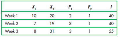
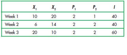
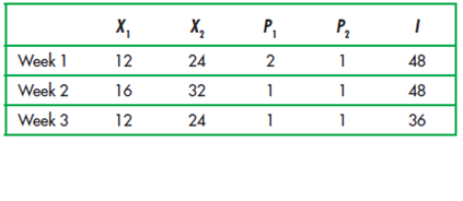
5. 5. Suppose that on every week, Bill, Mary, and Jane spend their whole weekly income for consuming two particular goods, x₁ and x₂. They consume these products to maximize their respective utilities.
      A. Here is Bill’s choice for three weeks.

Explain if Bill’s utility increases or decreases between i) week 1 and week 2; ii) week 1 and week 3. Put a graph for illustration.

        B. Next, consider the choices that Mary has made.

What is Mary’s utility increase or decrease between week 1 and week 3? Are these two goods are normal goods for Mary?

       C. Now, see the choices of Jane in this table.

Draw a budget line-indifference curve to depict Jane’s three chosen bundles. Study Jane’s preference in this situation. If there is a change in price for x₁, what will be the income and substitution effect?

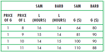
6. Sam and Barb, acquire utility from two things, the hours of leisure (L) and a number of goods (G) they consume. To maximize this utility, they are instructed to divide the 24 hours of a day between leisure hours and working hours. It is supposed that all hours are not spent working and leisure hours. The price of per unit good is $1 and for leisure, the price is the hourly wage.

Now examine the given table carefully and illustrate the two people’s leisure demand curve. (For vertical axis – price, for horizontal axis-leisure) Explain the difference between these two curves.

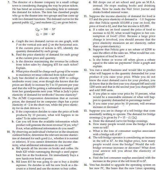
7. To modify the way of ticket pricing, the director of a theater company has hired an economic consultancy firm. The firm has classified two groups of people after considering the demand for tickets with two demand functions. The demand curve equation for this two groups are given below: (Q_gp – general public; Q_s – students)

Q_gp = 500 – 5P

Q_s = 200 – 4P

A. Placing P on the vertical axis and Q on the horizontal axis, draw two demand curves in one graph. Assume the current ticket price is $ 35. Calculate the quantity demanded each group.
B. What is the price elasticity of each group for current price and quantity?
C. Analyze if the director is maximizing the revenue if the ticket price is $35.
D. If he wants to maximize revenue collection, what should be the estimated price of a ticket for each group?

8.    Judy has decided to spend exactly $500 for college textbooks every year. It is known to her that the prices can rise 5 to 10 percent per year. She is going to get a considerable monetary gift from her grandparents next year. Calculate her price and income elasticity for textbooks.

9.    Suppose, the AMCE Corporation’s present demand for its computer chips carries the price elasticity -2 in short run for the current price. The price elasticity for its disk drive is -1.
a.    Now, if the corporation increases the price of both products by 10 percent, what will be the effect on the sales and sales revenue?
b.    Try to tell which product will return more revenue. Mention if any extra information is needed for this answer.

10.    Some information is given below about an individual. Study them and find out the appropriate income elasticity for each good. The goods can be normal or inferior. Mention if you need any additional information.
a.    The total income of Bill goes to the purchasing of books and coffee. He has found $20 from a paperback bin at the bookstore. He purchases a poetry book immediately.
b.    Bill has decided to buy a double espresso but he loses $10. He thinks that he will sell the new book at a discount to his friend to get money for buying coffee.
c.    When the price of book and coffee increase by 25 percent, Bill cuts down his consumption of both these goods by the same percentage.
d.    After dropping out of art school, Bill gets an M.B.A. He now reads the Wall Street Journal and drinks mineral water.

11.    Felicia spends $10,000 per year to buy food for her. Her income is $25,000 and price of food is $2. It is given that income elasticity for food is 0.5 and price elasticity of demand is -1.0.

a.    If after imposing a sales tax, the price of food increases to $2.50, what will be the change in consumption of Felicia? (Note: A large price change has occurred, therefore the price elasticity will measure an arc elasticity, not a point elasticity )
b.    If she gets a rebate of $2500 to ease the tax effect, what will be the consumption then?
c.    What do you think about the rebate that is equal to the sales tax payment? Is it better or worse? Explain with a graph.

12.     Think that you run a small business and have decided to know the effect of rising of the price on quantity demanded of your product. Assume that, you do not know about the demand curve for your product. On the first year, you sold 1200 unit, the unit price is $ 45. On the second year, the quantity is 1800 unit and price is $30 for each.
a.    What will happen to quantity demanded in percentage terms if you raise the price by 10 percent? Will it be a reasonable estimate?
b.    Calculate your revenue increase or decrease for the above decision.

13.    Assume that you are in charge of a toll bridge. The operating cost is nil. The demand for bridge crossing Q is
P = 15 – (1/2) Q
a.    Depict the demand curve for bridge crossing.
b.    Calculate the number of people who will cross the bridge if there is no toll.
c.    If the bridge toll is $5, what will be the loss in consumer surplus?
d.    If you charge $7 for bridge toll, how many people will use the bridge now? Check if the revenue increases or decreases. Also, find the elasticity of demand for it.
e.    Calculate the lost consumer surplus when the tax has been increased to $7.

14.     Vera has decided to upgrade the operating system on her PC. After asking her friends she finds out that Linux is technologically better than Windows, but it (Linux) costs more. She also notices that a few copy of Linux is available in the store. She goes for Windows. Explain Vera’s decision critically.

15.     You are the consultant of an agricultural cooperative, which is working on if their members should decrease their production of cotton in half next year. Your advice is needed to decide for the increment of member’s revenue. You know about the competence of both Cotton (C) and Soybean (S). According to you, the demand for cotton is C = 3.5 – 1.0 Pc + 0.25 Ps + 0.50I [Pc is the price of cotton, Ps is the price of soybean and I = income] Is the plan acceptable? Do you need any additional information? Mention it.

 

 

Links of Previous Main Topic:-

• Introduction Markets and Prices Preliminaries
• The Basics of Supply And Demand
• Consumer Behavior
• Appendix to Chapter 4 Demand Theory a Mathematical Treatment

Links of Next Microeconomics Topics:-

• Uncertainty and Consumer Behavior
• Production
• The Cost of Production
• Production and Cost Theory   A Mathematical Treatment
• Cost in the Long Run
• The Cost of Production Production with Two Outputs
• Profit Maximization and Competitive Supply
• The Analysis of Competitive Markets
• Market Power Monopoly and Monopsony
• Monopolistic Competition and Oligopoly
• Game Theory and Competitive Strategy