Solution of Assignments

1. Complete Enumeration Method

In this method of assignment problems, the cost for all the possible assignments has been carried out. After this, the solution with minimum cost will be taken as the optimal solution. This method can be used for smaller problems. This is because when the problem becomes complex, it will be hard to work out on a large number of alternatives to find out the optimal solution.

2. Simplex Method:

Minimize or Maximize,

Z = _ijC_ij

In simplex method, the simplex algorithm will be used. Thus, we subject to constraints,

1. _ij + _i2 + …………+ _in =          1
2. _ij + _2i + …………+ _nj =          1
3. _ij= 0 or, 1 for all values of i and j

It can be seen that there are ‘n’ x ‘n’ decision variables and ‘n’ + ‘n’ = 2n equalities. For solving assignment problems using this method; we can get that for 8 workers/jobs, there will be 64 decision variables and 16 equalities. All these need to be solved to find out the accurate solution. It can also be called as an extremely cumbersome method.

3. Transportation Method:

As the assignment problems are the special case of transportation model, it is also possible to solve the problems by transportation method. For this, we have already discussed optimality test in transportation problems.

This method requires n + n – 1 = 2n = 1 basic variables. Moreover, the solutions will severely degenerate. For the assignment problems, only ‘n’ basic variable will be there in the solution. Thus, for solving an assignment model, a very large numbers of dummy allocations will be made by using transportation method. Actually, this makes it very inefficient method to compute.

4. HAM or Hungarian Assignment Method (Minimization Case):

This method is also known as Flood’s Technique or Reduced Matrix Method. It was developed by the Hungarian Mathematician, D Koning. This method is considered as more simpler and more efficient method for solving assignment problems. This is because of its simple ways to find an optimal solution.

Following steps should be followed to use Hungarian Method:

Step 1: Formulate the opportunity cost table by using the following method

1. Subtract the smallest number present in each row of original cost matrix
2. Subtract the smallest number present in each column of the table that is obtained at (a.) above from every number in that column

Step 2: Make the assignments in the following manner

1. Examine each row while looking for a row with exactly one unmarked zero that will be in a square ( ) as the assignment will be made Cross ( X ) all other zeros in the cost matrix column. There will not be any assignment in future. Now, proceed in this way for all rows.
2. Examine all columns to find exactly one marked zero. Make an assignment at this point and put a square () here. Cross ( X ) all other zeros in the corresponding rows as no further assignments will be made. Now, proceed in this way for all columns.
3. The above (a.) and (b.) operations will be repeated till,
4. All zeros in the rows/ columns should be put in square ( ) or cross ( X ). Thus, there will be only one assignment in each row and each column. If this happens, it will be the optimal solution.
5. If some of the rows/ columns left without assignment, proceed to Step 4.

Step 3: Revise the opportunity cost matrix

1. Marking (√) all the rows that have no assignments
2. Marking (√) all the columns that have zeros but it haven’t marked earlier
3. Marking (√) all the rows that have assignments but it haven’t marked earlier
4. Repeat Step 3 (a.) and (b.) until there is no more row and column that could be marked.
5. Draw a straight line through each marked column and each unmarked row.

Step 4: Write a newly revised opportunity cost matrix

The initial opportunity cost matrix may not give an optimal solution. This is the reason we have to revise the table to find more zero costs from the present location to a newly uncovered location. For this, we have to subtract the smallest number in the matrix which is not covered by the straight line from all the other numbers that are not covered by the straight line (whether horizontally or vertically). Now, add this smallest number to every other number that is available at the intersection of the two straight lines (including the zeros).

Step 5: Repeat Step 2 and Step 4 until the optimal solution is achieved

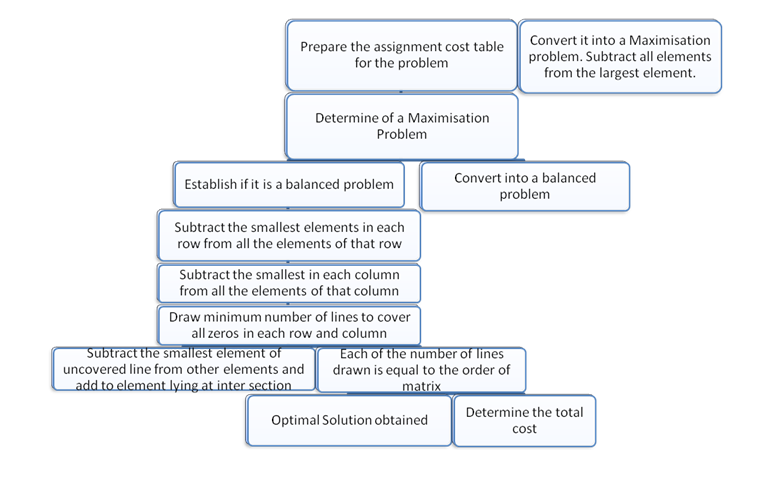
The above five steps are shown below in the form of a flow chart:

Prepare the assignment cost table for the problem  |

Convert it into a Maximization problem. Subtract all elements from the largest element. |

Determine of a Maximization Problem |

Establish if it is a Balanced Problem |

Convert into a Balanced Problem |

Subtract the smallest elements in each row from all the elements of that row |

Subtract the smallest in each column from all the elements of that column |

Draw minimum number of lines to cover all zeros in each row and column |

Subtract the smallest element of covered line from other elements and add to element lying at inter section |

Each of the number of lines drawn is equal to the order of matrix |

Optimal Solution Obtained |

Determine the Total Cost

PRACTICAL STEPS ARE INVOLVED IN SOLVING THE MINIMIZATION MAXIMIZATION

Links of Previous Main Topic:-

• Linear programming learning objectives and outline of chapter
• Introduction learning objectives
• Duality in linear programming
• Learning objectives
• Learning objectives and chapter outline in assignment model

Links of Next Finance Topics:-

• Minimization problems
• Learning objectives the transportation problems
• Special case of traveling sales man problem
• Replacement theory learning objectives and chapter outline

Customer Reviews